When a LiDAR publish rate falls below its configured frequency, first establish which rate you are measuring. Sensor packets arriving at the network interface, clouds emitted by the driver, callbacks received by an application, and frames drawn on screen are separate observations. A low number at the last stage does not identify a fault at the first. Increasing the frequency setting before locating the loss can make the experiment harder to interpret.
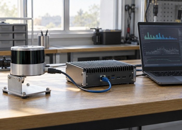
The useful starting point is a stationary, repeatable scene with one sensor and the smallest working software chain. Preserve the current configuration, measure each boundary over the same interval, and then add the normal processing load. This gives a robotics team evidence for deciding whether to investigate transport, cloud assembly, middleware reception, or application scheduling.
Keep hardware selection separate from runtime diagnosis. The LiDAR scan-rate and robot-fit guide helps define the required update behavior; the procedure below checks whether the installed integration delivers that behavior. It is a diagnostic plan, not a benchmark for any particular sensor.
Define four rates before changing a parameter
Write the configured publication target next to the exact parameter name, driver revision, sensor model, firmware, ROS distribution, and host operating system. Also record whether the driver emits one topic per sensor or combines devices. A launch-file value is an intended setting; it is not a measurement of packets, points, or successfully processed clouds.
An official open-source driver reference, for example, separates publication frequency from output format. Treat such documentation as specific to its supported hardware and revision. Do not copy another driver’s numerical limit into your system, and confirm the effective runtime configuration rather than assuming the edited file was loaded.
| Boundary | Record | Do not confuse it with |
|---|---|---|
| Sensor link | Packets and bytes arriving on the selected interface | Complete cloud messages |
| Driver output | Cloud count, point count, and publication timestamps | The launch-file target |
| Consumer input | Received callbacks and queue behavior | Successfully completed processing |
| Application output | Completed jobs and end-to-end age | Display refresh or render rate |
These quantities can legitimately differ. A cloud may contain many packets; a consumer may deliberately process only selected clouds. Decide which boundary the application actually requires before calling the integration slow. For navigation, message freshness can matter as much as average throughput.
Capture a quiet baseline at the sensor link
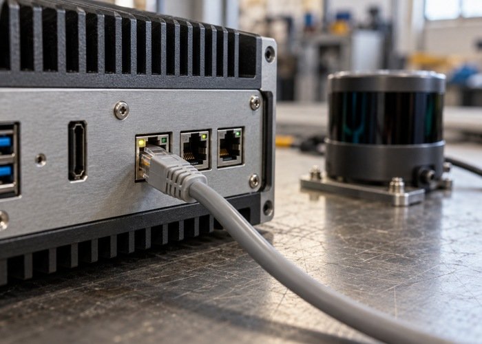
Use a known static target and retain the same sensor configuration throughout the baseline. Close unnecessary viewers and avoid running several diagnostic subscriptions at once. Document the interface, addresses, destination ports, cable path, and whether the driver runs directly on the host or inside a container. If no data reaches the driver at all, follow the separate viewer-versus-driver reception checks first.
Take interface counter snapshots at the start and end of the measurement interval. The Linux interface-statistics documentation explains why received, dropped, missed, and driver-specific counters do not all describe the same event. Work with counter changes during the test, and record their names and collection method. A historical nonzero counter does not establish current loss.
A packet capture can show arrival spacing, burst structure, and whether the expected stream reaches the chosen interface. The tcpdump reference also distinguishes captured packets from drops reported by the capture mechanism. A capture with its own drops is incomplete evidence; a clean capture still does not prove that the driver socket accepted every packet.
Measure driver emission without adding a heavy consumer
Prefer a lightweight, bounded counter at the publication boundary when the driver offers one. If source instrumentation is practical, count emitted messages and points rather than writing every point to a terminal. Save the observation interval and clock used. Exclude startup behavior from a steady-state comparison, but keep startup logs as a separate record.
The ROS 2 Jazzy topic-rate tool implementation describes its result as a subscriber receiving rate that can be affected by resources and QoS. Therefore, ros2 topic hz /your_cloud_topic is useful evidence from one observer, not direct proof of the driver’s internal emission frequency. Check the installed tool’s help because options and behavior vary between distributions.
Compare the observer’s message type and endpoint policies with the actual publisher. A silent or selective subscriber needs a compatibility investigation, such as the ROS 2 LiDAR QoS mismatch procedure, before its count can be treated as a rate measurement. Avoid changing QoS, batching, and processor settings together; that removes the ability to explain an improvement.
Keep message rate and point throughput together
A higher message count can result from smaller batches without increasing the number of measurements available to the application. Record points per cloud, total points received over the interval, empty clouds, and the distribution of inter-message gaps. Average frequency alone hides bursts followed by pauses. Preserve representative timestamps so another engineer can reconstruct the observation.
Compare the raw stream with the consumer’s input before filtering or downsampling. Changes in point-cloud processing can alter the amount of work and the output point count. That may be deliberate application behavior. Label every counter by stage so an output filter is not mistaken for a sensor losing measurements.
Add load one component at a time
After the quiet baseline, enable recording, visualization, mapping, and other consumers individually. For each step, use the same scene and observation interval, then return to the baseline. Log received callbacks separately from completed processing jobs. If callbacks arrive normally but completed jobs fall behind, examine processing time and queue age before changing the sensor.
On Jetson platforms, the version-specific tegrastats documentation provides a reference for resource telemetry. Correlate available load, frequency, memory, and temperature observations with the pauses. An aggregate CPU percentage is insufficient by itself: the delayed task may depend on one busy thread or another constrained resource.
Build an evidence worksheet that supports the next decision
For each run, save the configuration identifier, active components, start and end times, packet-counter deltas, emitted clouds, received clouds, completed jobs, point totals, and longest observed gap. Add the data source for each number. The worksheet should make missing measurements explicit rather than filling them with estimates.
A stable link with fewer driver emissions points toward assembly or publication scheduling; stable emissions with fewer consumer callbacks points toward reception or observer behavior. Normal callbacks with delayed completed work points toward application capacity. These are investigation paths, not diagnoses established by one row. Repeat the change and its reversal before deciding that it explains the symptom.
For an illustrative comparison, use a fixed scene and a chosen test interval, run the driver alone, then enable the recorder, and finally restore the original state. No universal acceptable percentage is implied. Define acceptance from the application’s freshness and throughput needs. A simulation-based integration plan can help set those needs, while the hardware trial checks the actual pipeline.
Questions before changing the publish frequency
Should I increase the setting to compensate for a low observed rate?
Only after identifying the limiting boundary and confirming the supported range for the exact sensor and driver. Otherwise a higher setting can change batch size or increase overhead without addressing the measured delay. Keep the original configuration so the result can be reversed and compared.
Does a clean network capture clear the driver?
No. It demonstrates what the capture observed at one interface. The driver still has to receive, decode, assemble, and publish the data. Combine capture evidence with driver-side counts and consumer observations before assigning responsibility.
What should I send for integration support?
Send the version list, sanitized configuration, short representative trace, counter worksheet, and a description of the smallest repeatable load change. This makes a LiDAR publish-rate investigation actionable and avoids replacing hardware on the strength of a single terminal reading.