Conveyor belt LiDAR profiling works because light travels at a fixed speed — and modern sensors can exploit that fact thousands of times per second to build a complete three-dimensional map of every object that passes beneath them.
Time of Flight (ToF) explained: A ToF sensor fires a laser pulse, that pulse strikes a surface, and the sensor measures the precise time elapsed before the reflected light returns. Because the speed of light is constant, distance equals half the round-trip travel time multiplied by c. Repeat this across hundreds of scan lines and you get a dense point cloud — not a flat silhouette.
The difference between 2D scanning and 3D profiling matters enormously in practice. A conventional 2D laser scanner captures a single planar slice of a passing object, producing a cross-sectional outline. As the conveyor carries the item forward, successive slices are stitched together using belt-encoder feedback to reconstruct a three-dimensional shape. That stitching process is where pulse frequency becomes critical. If a sensor fires too slowly relative to belt speed, the gap between successive scan lines grows wide enough to miss surface detail — a sagging polybag side wall, a crushed corner, a protruding label. According to the Material Handling Institute, integrating LiDAR into automated sortation systems enables real-time data acquisition at belt speeds exceeding 2.5 meters per second without sacrificing data density. At that throughput, sensors typically need pulse repetition rates in the hundreds of kilohertz range to maintain sub-centimeter resolution across the full parcel profile.
Inline profiling — measuring objects while they move — stands in direct contrast to static dimensioning, where a parcel is stopped, placed on a reference surface, and measured from a fixed vantage point. Static systems are accurate but slow; inline systems must reconcile motion, vibration, and irregular geometry simultaneously. That is precisely why the fundamental physics of ToF sensing underpins every high-throughput dimensioning deployment worth considering.
That last challenge — handling geometry that defies simple bounding boxes — is where the real complexity begins, particularly for soft-shell and polybag shipments.
Solving the ‘Irregular’ Problem: Polybags and Crushed Parcels
Traditional dimensioning sensors treat every package as a perfect rectangular box — and that assumption is precisely where they break down at scale.
Light curtains and 2D laser scanners calculate dimensions by projecting a bounding box around whatever they detect. For a rigid cardboard carton, that shortcut is close enough. For a polybag slumping to one side or a return shipment with a crushed corner, the “boxing error” inflates the measured volume dramatically, generating incorrect dimensional weight charges and downstream sortation mismatches. An automated parcel dimensioning system built on these legacy sensors simply cannot distinguish between the actual surface of a soft-shell package and the invisible rectangular envelope it projects around it.
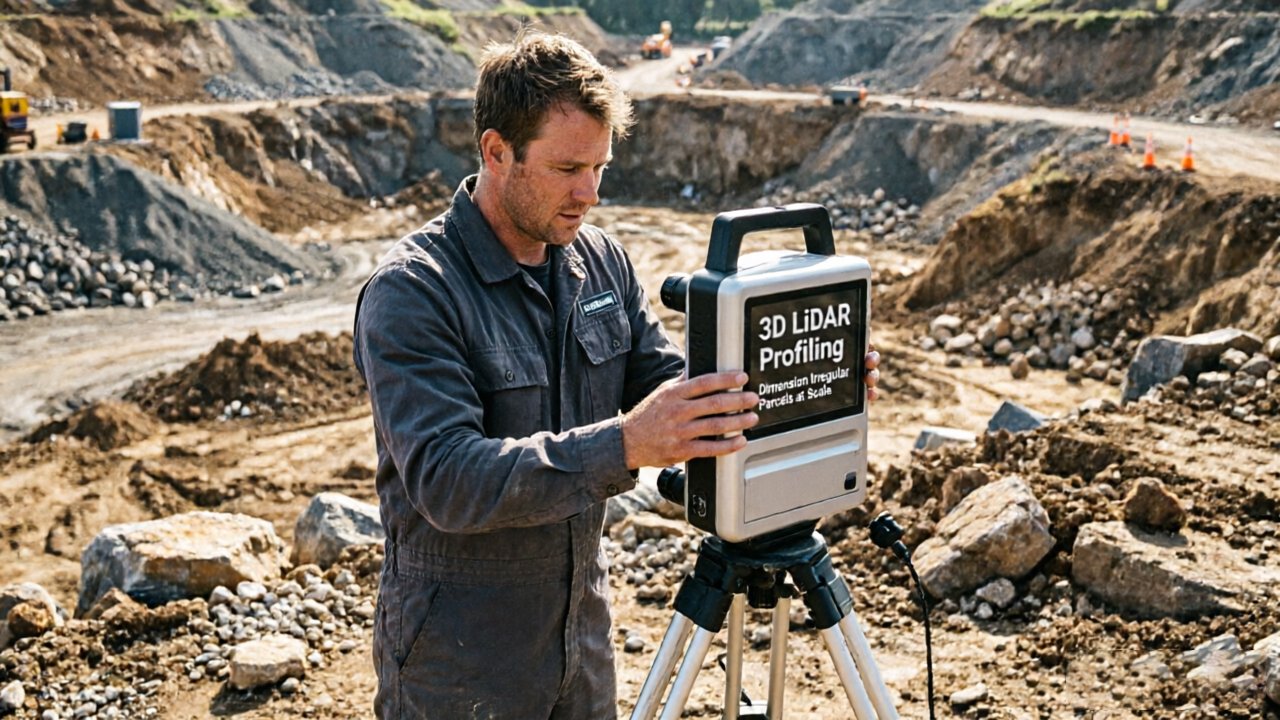
3D LiDAR solves this by capturing the exact geometry of each object — not a guess at its outer boundary. As noted by Parcel and Post Technology International, 3D LiDAR generates a dense point cloud that records the true shape of irregular items like polybags and crushed parcels, surfaces that traditional light curtains fundamentally fail to measure. The difference is not marginal: a polybag can read 30–40% larger than its actual displaced volume when bounding-box methods are applied.
Point cloud density is what makes sub-centimeter accuracy achievable. Higher line rates and angular resolutions produce denser returns per square centimeter of surface, which matters most on curved or collapsed packaging where sparse data would smooth over real deformations. Understanding the underlying sensing architecture — particularly how ToF and FMCW approaches compare — helps explain why some wavelengths outperform others on low-reflectivity materials like matte black poly film.
Surface reflectivity adds another layer of complexity. Common failure modes of traditional sensor types include:
- Specular reflection from glossy packaging causing missed returns in structured-light systems
- Low-contrast edges on transparent film confusing 2D cameras and light curtains
- Material absorption at certain wavelengths reducing signal strength on dark polybags
- Surface sag in soft packaging creating depth variation that 2D sensors register as a flat plane
- Partial occlusion from overlapping parcels triggering single-object false reads
These are exactly the real-world variables that make bulk flow measurement — where material shapes are even less predictable — a compelling next frontier for 3D profiling technology.
Online Measurement Methods for Material Flow and Bulk Volume
LiDAR profiling doesn’t stop at discrete parcel dimensioning — it also solves one of industrial logistics’ harder problems: measuring continuous, irregular material flowing across a belt in real time.
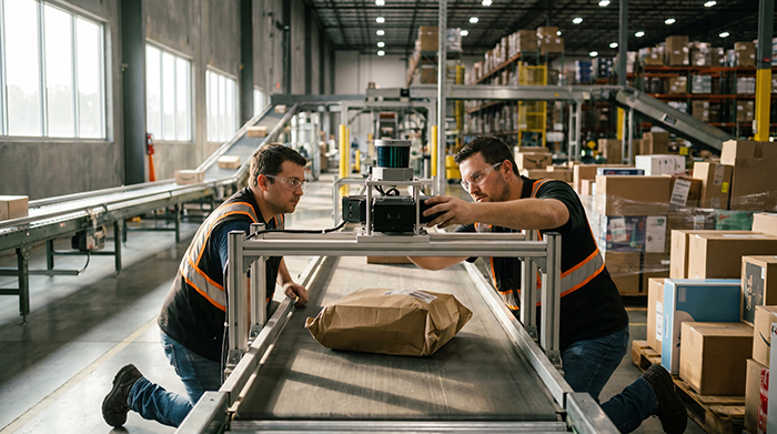
Where a parcel dimensioning system handles individual units, bulk flow measurement requires integrating cross-sectional geometry across a moving stream. The core formula is straightforward: Volume Flow Rate = Cross-Sectional Area × Belt Velocity. A LiDAR sensor mounted above the conveyor captures a 2D profile slice of the material pile. Multiply that instantaneous cross-section by the known belt speed, and you get a continuous volumetric flow estimate — updated with every scan cycle.
In practice, this process involves three steps working in sequence. First, the sensor captures a height profile across the full belt width. Second, the software calculates the cross-sectional area by comparing the loaded profile against the baseline empty-belt reading. Third, that area value is multiplied by the real-time belt velocity signal from an encoder, yielding a running volume total. LiDAR-based systems can achieve measurement accuracies of ±0.5 inches or better on fast-moving lines, according to industry benchmarking data from Logistics Management.
Real-time density estimation extends this further. When bulk density values are known — or sampled periodically by a loadcell — operators can convert volume flow directly into mass flow, enabling continuous tonnage monitoring without halting production. This is especially valuable in applications where material composition shifts, such as mixed-grade ore or wet agricultural grain.
The practical reach of this method spans mining, grain handling, quarrying, and bulk freight terminals — anywhere a belt carries loose or semi-loose material at scale. The underlying time-of-flight sensing principles that make per-parcel profiling accurate are the same ones enabling sub-second refresh rates in these demanding bulk environments.
This measurement approach works cleanly for uniform overheads — but when material piles high or shifts to one side, a single sensor can miss critical geometry. That’s exactly the blind-spot problem that multi-sensor configurations are designed to address.
Eliminating Shadowing: Multi-Sensor Configurations and Placement
A single overhead LiDAR sensor creates blind spots that distort dimensional data — and for high-profile or angled parcels, those blind spots can invalidate an entire scan.
The “shadowing” effect is the core limitation of single-sensor dimensioning systems. When a scanner fires from directly above, tall or leaning objects cast geometric shadows — regions where no laser pulse ever reaches. The result is a point cloud with missing flanks, undercut bases, or entirely absent side faces. For a perfectly rectangular box moving flat on a belt, this matters little. For the polybags and irregular freight discussed earlier, it’s a fatal flaw.
Strategic sensor placement transforms this weakness. Three configurations address shadowing at different levels of severity:
- Overhead mounting captures top-face geometry cleanly and serves as the primary reference plane. It’s the starting point for most dimensioning tunnels but insufficient on its own for objects taller than roughly 20–25 cm.
- Side-mounted sensors fill vertical faces. Placed at conveyor height or mid-profile, they capture the lateral geometry that overhead units miss entirely — critical for cylindrical objects or parcels stacked at an angle.
- Dual-diagonal configurations combine angled sensors above the conveyor on both sides of the belt. This geometry is particularly effective for steep-sided or peaked objects, where neither a pure overhead nor a pure side view captures the full envelope.
As Inbound Logistics notes, by placing sensors at multiple angles — overhead and side-mounted — the system ensures that the blind spots of an irregular parcel are filled in. The practical result is a more complete point cloud with fewer interpolated gaps.
Multi-sensor synchronization is where architecture gets demanding. Each unit generates its own coordinate frame, so fusing streams requires precise extrinsic calibration — translating every sensor’s data into one shared spatial reference. Timing synchronization matters equally; even millisecond offsets between scans create ghost edges when a parcel is moving. These same sensor-fusion principles apply across industries, as explored in multi-sensor depth applications beyond logistics.
The online measurement methods for material flow that work best at scale treat multi-sensor fusion not as a post-processing step but as a real-time operation, merging streams before any dimensional calculation begins. That architectural choice directly determines whether blind-spot compensation is accurate or merely cosmetic — a distinction that matters even more once belt dynamics enter the equation.
Characterizing Conveyor Belt Longitudinal Dynamics
Belt motion isn’t neutral background — it’s an active source of measurement error that 3D LiDAR point cloud dimensioning systems must account for explicitly.
Belt vibration introduces micro-displacement artifacts into scan data. As a sensor sweeps across a moving conveyor, even small oscillations — typically 1–3 mm in high-throughput environments — create positional smearing in the point cloud. The result is artificially inflated bounding boxes and degraded edge definition, particularly on low-profile parcels where the margin for error is smallest. As the MDPI Sensors Journal notes, identifying and characterizing conveyor belt longitudinal dynamics is critical for precise positioning and control in automated unloading systems — and the same principle applies directly to dimensional accuracy.
Belt noise filtering separates legitimate object returns from surface-level interference. In practice, this means establishing a dynamic ground plane that updates continuously as belt wear and surface irregularities shift the baseline. A worn belt may sag 4–6 mm between idlers; without compensation, that sag registers as object geometry. Effective filtering algorithms model the belt surface independently, subtract it from each scan frame, and flag anomalies that exceed expected variance thresholds.
Technical Tip — Encoder Synchronization: Pairing your LiDAR unit with a belt encoder is non-negotiable for spatial accuracy. The encoder feeds real-time velocity data to the scan processor, which uses it to assign precise longitudinal coordinates to every point. Without encoder integration, belt speed variation — even ±2% — compounds into positional drift that corrupts length measurements over distances greater than 300 mm. For conveyor applications, single-line ToF sensors operating in synchronized mode provide a reliable trigger reference alongside your 3D profiling head.
Compensating for surface irregularities requires periodic recalibration routines, especially in environments where belt replacement cycles stretch beyond 12 months. A common pattern is to run an empty-belt calibration scan at shift start, storing a fresh reference surface. This keeps the subtraction model current and prevents accumulated drift from propagating into DIM data.
With the belt dynamics cleanly characterized and filtered, the scan stream becomes a reliable foundation for the next layer of automation — counting, classifying, and tracking individual items as they move through the system.
Automated Object Counting and Tracking Integration
Dimensioning accuracy means little if the system can’t reliably separate, classify, and hand off each parcel to the broader logistics workflow in real time.
LiDAR-based separation detection solves one of the most persistent problems on high-speed conveyor lines: identifying where one item ends and another begins. Point cloud segmentation algorithms continuously analyze the incoming 3D scan data, detecting gaps between objects and flagging parcels that have merged or overlapped during transport. Unlike camera-based approaches that struggle with color-uniform backgrounds, LiDAR’s depth-first geometry makes separation decisions based purely on spatial discontinuity — far more reliable in variable lighting conditions.
Item classification adds the next layer of intelligence. Research into automated conveyor belt object counting using integrated LiDAR demonstrates that convolutional networks can classify items — box, polybag, or flat envelope — directly from point cloud geometry. This distinction matters for irregular object volume calculation: a rigid carton tolerates a tight bounding box approximation, while a soft polybag demands a conforming mesh approach to avoid systematic volume overreads that erode billing accuracy.
WMS Integration is where this data converts into operational value. Once a parcel is dimensioned and classified, the system pushes a structured data record — dimensions, weight, item type, and timestamp — directly to the Warehouse Management System via API or message queue. This record triggers downstream sortation rules, label printing, and slotting assignments without manual intervention. The sensor’s time-of-flight precision, similar in principle to the distance-mapping techniques used in autonomous systems, ensures the data packet arrives with sub-centimeter dimensional fields that WMS routing logic can act on immediately.
Tracking through blind zones — the physical gaps between sensor arrays — relies on belt encoder data synchronized with the LiDAR scan timestamps. As items transit these gaps, predictive handoff logic maintains parcel identity continuity, ensuring the WMS record stays attached to the correct physical object through the full sortation run. That data integrity, maintained from first scan to final sort, is precisely what makes it defensible for billing and dispute resolution — a point the next section examines in detail.
The ROI of ‘Legal for Trade’ Volumetric Accuracy
Precise volumetric data isn’t just a technical achievement — it’s a direct line to recovered revenue, reduced disputes, and smarter operational decisions across the logistics chain.
Dim weight leakage is one of the most underestimated cost drivers in parcel shipping. When a 3D LiDAR system captures accurate bounding-box dimensions for irregular parcels — polybags, over-wrapped pallets, oddly shaped returns — carriers can bill dimensional weight with confidence instead of approximating. Manual or 2D measurement methods routinely underestimate volume on non-rectangular shapes, leaving revenue on the table with every shipment. At scale, even a 2–3% improvement in dim weight capture accuracy translates to meaningful top-line recovery.
Dispute resolution is where defensible data earns its keep operationally. When a shipper challenges a carrier’s volumetric charge, having a timestamped 3D point cloud tied to a specific parcel ID, belt encoder position, and WCS event log changes the conversation entirely. As noted by Logistics Management, LiDAR profiling provides the precision necessary for “Legal for Trade” certification, ensuring that shipping charges based on volumetric weight are accurate and legally defensible — not just internally auditable, but externally challengeable in a dispute context. That certification status is increasingly a requirement rather than a differentiator for high-volume fulfillment operations.
Beyond billing, precise volume data feeds two additional operational improvements worth highlighting:
- Truck loading optimization: Accurate cubic dimensions allow load-planning algorithms to maximize trailer utilization, reducing dead space and lowering cost-per-shipment.
- Warehouse slotting: Knowing true parcel dimensions enables smarter slot assignments, reducing re-slotting events and pick path inefficiencies.
- Maintenance and calibration overhead: Certified systems require scheduled recalibration — typically tied to production shift cycles — to maintain Legal for Trade tolerances. This is a real operational cost, though it’s predictable and far smaller than the revenue leakage it prevents.
Understanding how these business outcomes connect to sensor-level decisions — from pulse-based ranging principles to multi-sensor configurations — is what separates a well-integrated dimensioning investment from a point solution that underdelivers. The next section distills everything into the core takeaways worth carrying forward.
The Bottom Line: Key Takeaways for LiDAR Dimensioning
3D LiDAR profiling isn’t a luxury upgrade — it’s the operational baseline any modern fulfillment center needs to dimension irregular parcels accurately, compliantly, and at scale.
The previous sections have built a thorough case across sensing physics, multi-head geometry, WMS integration, and revenue recovery. Here’s what ties it all together:
- Irregular objects demand 3D profiling. Polybags, padded mailers, and oddly shaped bundles collapse or bulge unpredictably on a conveyor. Traditional 1D or 2D sensors produce bounding-box estimates that routinely overstate or understate true volume. Only a dense 3D point cloud can capture the actual surface geometry of a non-rigid parcel.
- Multi-sensor coverage is non-negotiable. A single profiler leaves shadow zones — areas occluded by the parcel’s own geometry or by adjacent items. Staggered, multi-angle sensor arrays eliminate those blind spots and deliver the 360-degree volumetric closure that billing accuracy requires.
- High-frequency ToF enables real-world throughput. Time-of-Flight measurement technology operates at pulse rates fast enough to capture full profiles even when belts exceed 2.5 m/s. According to Peerless Media, LiDAR systems can maintain ±0.5 inch accuracy at high sortation speeds — a tolerance tight enough to satisfy Legal for Trade certification requirements.
- Integration converts data into decisions. Raw distance readings become logistics intelligence only when synchronized with encoder pulses and pushed into WMS or TMS platforms. That pipeline — from photon return to rated shipment charge — is what transforms a hardware investment into measurable ROI.
The core principle: precision at the sensor level multiplies across every downstream process it touches — from carrier invoicing to cube utilization to returns management.
With the strategic case established, practical deployment questions naturally follow. How does ambient warehouse light affect scan quality? Can LiDAR read through shrink-wrap? What does a real calibration schedule look like? The next section addresses those implementation realities head-on.
Implementation FAQ: Deploying LiDAR on the Line
Deploying inline LiDAR dimensioning raises practical questions that every ops team encounters — and getting the answers right separates a smooth rollout from a costly retrofit.
Ambient light interference is the most common first concern. Modern 3D LiDAR sensors use specific wavelengths engineered to minimize interference from warehouse lighting and highly reflective surfaces, per LidarStar Technical Support. In practice, overhead fluorescents and even high-bay LEDs rarely disrupt a properly configured profiler. The key mitigation steps are mounting the sensor at a controlled angle, shielding the scan zone from direct sunlight exposure near dock doors, and selecting a sensor whose operational wavelength sits outside the visible spectrum.
Transparent packaging is a legitimate challenge, not a dealbreaker. Shrink-wrap and clear poly bags scatter rather than reflect a clean return signal, which can introduce minor dimensional noise. One practical approach is pairing the LiDAR scan with a short conveyor gate that compresses loose wrap against the parcel before the scan window — reducing measurement variance without slowing throughput. FMCW-based sensors offer improved coherent detection that handles low-reflectivity surfaces better than standard time-of-flight alternatives.
Calibration intervals depend on throughput and environment. Most inline profilers require a full geometric calibration every 90 days under normal warehouse conditions, with a quick reference-target check at shift start. High-vibration environments — near sorters or slam lines — benefit from monthly verification cycles. Skipping calibration is the single fastest way to erode the legal-for-trade accuracy your billing rates depend on.
For teams evaluating sensor performance before purchasing, a video walkthrough of the profiling process in action provides concrete context that spec sheets alone cannot deliver. Watch this demonstration of 3D LiDAR annotation precision:
Seeing the point cloud resolve around an irregular parcel in real time makes the business case tangible. The technology is mature, the integration paths are well-documented, and the revenue recovery starts the moment the first mis-dimensioned package is caught. The only remaining question is how many billing cycles to wait before acting.