A single horizontal laser slice cannot protect an AMR from a world that extends in three dimensions — and in busy warehouses, that gap between what a sensor sees and what actually exists is where collisions happen.
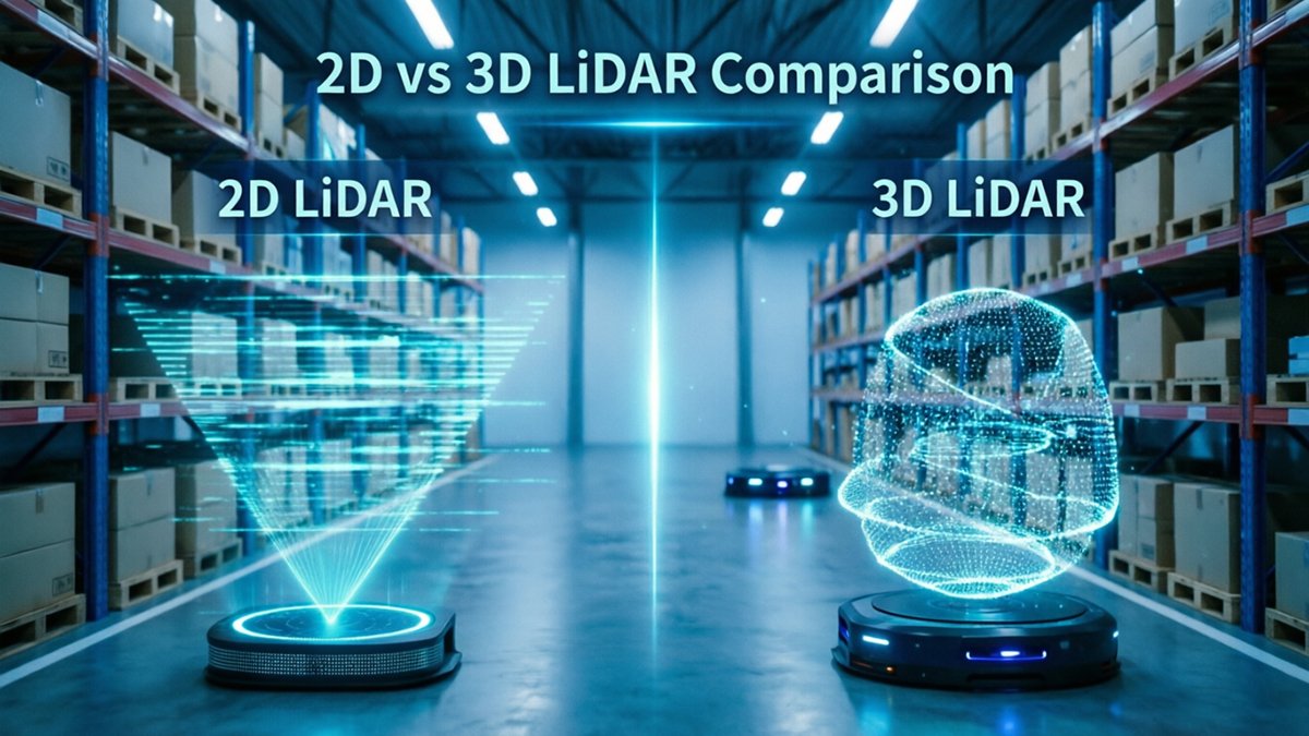
2D LiDAR’s fundamental flaw is its physical blind spot: it scans one fixed plane, typically 15–30 cm above the floor. Overhanging forklift tines sit above that plane. Low-profile pallets slide beneath it. Angled conveyor legs, protruding shelf brackets, and slumped cargo bags all exist in the vertical space a flat scan simply never captures. The robot perceives a clear path and proceeds — until it doesn’t.
Conservative path planning is the predictable downstream consequence. Without volumetric data, a well-tuned robot obstacle avoidance algorithm compensates for sensor uncertainty by increasing obstacle margins significantly. The robot slows, stops, and reroutes around perceived threats or widely overestimates clearances. In practice, this produces inefficient “stop-and-wait” cycles that erode throughput across an entire facility — a hidden operational cost that compounds daily.
The real-world stakes escalate in dynamic environments. Humans cross lanes unpredictably. Forklifts move inventory continuously. A 2D perception stack, no matter how sophisticated its software layer, cannot reason about an obstacle it physically cannot detect. Near-miss incidents and minor collisions follow, creating both safety liability and costly downtime. The challenge of spatial perception has only grown harder as warehouses densify their operations.
As Robotics Business Review states, “The transition from 2D to 3D LiDAR is the single most significant hardware upgrade for AMRs to achieve Level 5 autonomy in unstructured environments.” That upgrade starts with understanding what a full point cloud actually delivers — and how dense volumetric data transforms local planning from reactive to predictive.
Decoding the 3D Point Cloud: Volumetric Data for Local Planning
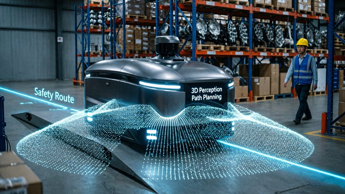
Three-dimensional point clouds give AMRs a complete spatial model of their environment — not just a flat cross-section, but a true volumetric picture of every obstacle in range.
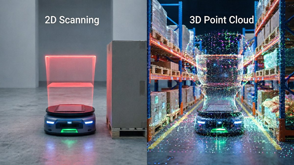
Point cloud density directly determines how much spatial truth a navigation stack can work with. A modern 3D LiDAR sensor fires thousands of laser pulses per second across multiple vertical channels, producing a dense field of (X, Y, Z) coordinate returns. The higher the point density, the finer the spatial resolution — meaning the system can distinguish the leg of a pallet jack from a support column, or detect a cardboard box left on a ramp before any wheel gets near it.
Raw point clouds, however, aren’t immediately useful. The navigation stack needs structure. What typically happens is a process called voxelization: the continuous point cloud is divided into a three-dimensional grid of uniform cubic cells — voxels — where each occupied cell signals a collision hazard. This transforms millions of scattered returns into a compact, queryable occupancy map that path planners can act on in real time. According to research into 3D obstacle detection pipelines, this approach preserves spatial accuracy while keeping computational load manageable.
Where 2D sensors capture only a horizontal slice — missing overhangs, low-clearance beams, and floor-level debris — 3D data captures the full volume of an obstacle, from base to apex. The robot doesn’t just know that something is in the way; it knows its complete shape and extent.
That richer geometry directly reduces costly stop-and-wait cycles. Instead of halting because a 2D sensor can’t classify an ambiguous return, the AMR uses volumetric context to find a navigable gap — keeping throughput moving. For effective AMR obstacle avoidance, LiDAR-derived voxel maps are what make that decisiveness possible.
This volumetric foundation also sets the stage for more sophisticated local planning — specifically, the trajectory optimization algorithms that determine how an AMR threads through a congested aisle.
Algorithm Deep Dive: DWA and TEB in 3D Environments
Local planning algorithms determine whether a robot navigates efficiently or gets stuck — and 3D LiDAR point cloud analysis is what gives both DWA and TEB their real competitive edge in dynamic environments.
Dynamic Window Approach (DWA) samples a window of feasible velocities and scores each candidate trajectory against clearance, goal alignment, and forward speed. In practice, DWA benefits enormously from 3D volumetric data because it can evaluate vertical clearance simultaneously with lateral clearance — ruling out paths that pass beneath a shelf overhang or too close to a forklift mast that a 2D slice would have missed entirely.
Timed Elastic Band (TEB) takes a different angle. Rather than sampling velocity space, TEB treats the trajectory as a sequence of poses that can be elastically “stretched” and “compressed” subject to time, distance, and obstacle proximity constraints. Because TEB reasons about the shape of the entire path, not just the next velocity command, it consistently finds tighter, more efficient routes around irregular 3D obstacles — the kind of confident, close-clearance bypass that would be unsafe to attempt with flat 2D awareness.
Key Insight: 3D spatial context enables both algorithms to execute tighter bypasses that are geometrically verified — not just assumed safe.
Handling dynamic obstacles is where real-time point cloud updates become critical. Humans and moving vehicles change position faster than any static map can represent. Both DWA and TEB can ingest continuous point cloud refreshes and re-solve trajectories mid-execution. Research cited in the Journal of Field Robotics shows this approach can reduce collision rates by up to 40% compared to vision-only or 2D-based systems in highly dynamic environments.
40% fewer collisions. That single figure makes the case for 3D-based local planning in any high-traffic facility.
Of course, the quality of these algorithms depends entirely on the sensor feeding them — which raises an important question about what kind of 3D sensor actually belongs on an AMR.
The 3D Camera vs. 3D LiDAR Debate for Obstacle Avoidance
Choosing between 3D cameras and 3D LiDAR for AMR obstacle avoidance isn’t a minor spec decision — it fundamentally shapes how reliably a robot performs under real-world conditions.
Passive sensing has a core vulnerability: cameras depend entirely on ambient light. In a warehouse environment, that means navigating deep shadows cast by racking systems, blinding glare near loading docks, and inconsistent lighting across shifts. Stereo vision and depth cameras struggle under these conditions, producing noisy or incomplete depth maps that can cause the DWA algorithm robotics teams rely on to plan around phantom obstacles or miss real ones entirely.
LiDAR’s active sensing advantage sidesteps this limitation completely. Because it emits its own laser pulses and measures return time, 3D LiDAR produces consistent, high-density point clouds whether the facility is fully lit or pitch dark. As outlined in this technical analysis of LiDAR-based obstacle detection, active sensing provides the kind of environmental independence that passive vision simply cannot match in high-stakes deployments.
There’s also a computational dimension worth examining:
- Stereo vision depth maps require significant processing to reconstruct geometry from paired image frames, introducing latency.
- LiDAR point clouds deliver pre-structured spatial data, reducing the processing burden for real-time local planning.
- Sensor fusion (LiDAR + Camera) is increasingly the gold standard — each sensor compensates for the other’s blind spots, a pattern validated by AMR perception research examining visual-data-driven platforms.
For teams building high-reliability AMRs, understanding how different LiDAR capture methods affect sensing consistency is critical. However, even the best sensor fusion setup has a ceiling — unless the robot can actually classify what it’s detecting, not just detect it. That distinction is where semantic segmentation changes everything.
Implementing Semantic Segmentation: Distinguishing Humans from Hardware
3D LiDAR’s real competitive advantage isn’t just detecting obstacles — it’s understanding what those obstacles actually are.
Moving beyond the binary “obstacle vs. no obstacle” model is what separates truly intelligent AMR navigation from basic collision avoidance. Traditional 2D LiDAR sees a point cluster and stops. Semantic segmentation sees a person — and responds accordingly. This distinction matters enormously in mixed-use warehouse environments where forklifts, pallet racks, conveyor legs, and workers share the same floor space simultaneously.
PointNet++ is the architecture making real-time classification practical. Developed through research at Stanford University’s Autonomous Systems Lab, PointNet++ processes raw 3D LiDAR point clouds hierarchically, grouping local point neighborhoods to extract geometric features at multiple scales. Critically, it can classify objects in real-time — distinguishing a static pallet rack from a moving worker within a single scan cycle. The TEB local planner LiDAR integration then uses these classifications downstream, dynamically adjusting trajectory cost functions based on object type rather than treating every detected point cluster identically.
Safety margins are where semantic awareness translates into real-world value. A robot navigating past a fixed shelving ux’anit can execute a tight bypass with minimal clearance. That same robot approaching a worker should automatically apply a wider safety buffer — accounting for unpredictable human movement and directional changes that static infrastructure simply doesn’t exhibit.
“Advanced algorithms like PointNet++ process LiDAR data to classify objects in real-time, allowing the AMR to choose a ‘tight’ bypass for a static object but a ‘wide’ safety margin for a moving person.” — Stanford University Autonomous Systems Lab
The throughput impact is measurable. Robots that over-cautiously treat every obstacle identically slow down at fixed infrastructure unnecessarily. Semantic awareness enables confident, faster navigation around predictable objects — while appropriately yielding to humans. As solid-state sensing technology continues maturing, these classification capabilities will only sharpen. Of course, all this rich semantic data creates a significant computational challenge — one that requires careful pipeline optimization to manage in real-time.
Overcoming the Computational Burden of 3D Data
3D LiDAR point clouds deliver unmatched spatial detail, but that richness comes with a real cost: raw data rates that can easily overwhelm an AMR’s onboard compute stack.
The single most effective first step is aggressive downsampling before any processing begins. Voxel grid filtering divides the point cloud into small cubic cells and retains only one representative point per cell. This dramatically reduces data volume — sometimes by 80% or more — while preserving enough geometric structure for reliable obstacle detection. Voxel-based R-CNN architectures build on this principle, optimizing 3D obstacle detection without overwhelming onboard compute resources, making them increasingly attractive for real-time AMR deployments.
Edge computing vs. centralized processing is a critical architectural decision. Running the navigation stack locally on the robot eliminates network latency, which matters enormously when avoiding a fast-moving forklift. Centralized processing offers more raw compute power but introduces round-trip delays that are unacceptable in dynamic environments. In practice, a hybrid approach works well: edge hardware handles time-sensitive filtering and collision detection, while heavier workloads — including semantic segmentation LiDAR pipelines — are offloaded to more capable processors when latency budgets allow.
ROS2 pipeline optimization deserves deliberate attention. Point cloud topics can flood the message bus if left unconfigured. Common techniques include:
- Throttling publish rates to match the navigation planner’s update frequency
- Using nodelet or component-based architectures to reduce inter-process serialization overhead
- Applying passthrough filters to crop irrelevant Z-axis data outside the robot’s operational plane
- Leveraging hardware-accelerated libraries (GPU-based CUDA kernels) for parallel point processing
Hardware acceleration is increasingly accessible. Modern solid-state LiDAR designs pair naturally with embedded GPU platforms, enabling real-time processing that was impractical just a few years ago. Getting the computational side right is, of course, only half the challenge — the physical integration of the sensor itself demands equal rigor, which the next section addresses directly.
Integrating 3D LiDAR: A Practical Implementation Guide
Moving from concept to deployment requires a disciplined, step-by-step approach — one that addresses sensor selection, physical mounting, software alignment, and validation before a robot ever enters a live environment.
Getting the hardware choice right from the start saves enormous rework downstream.
1. Select FOV for full coverage. A single forward-facing 3D LiDAR leaves flanks and rear quadrants exposed. In practice, 3D mechanical and forward-facing sensors are often combined with blind-compensation sensors to deliver 360-degree volumetric coverage. Map your robot’s geometry first, then identify which angular gaps require supplemental units.
2. Choose sensor technology for your environment. Mechanical LiDAR offers wide vertical FOV and proven field reliability but carries more moving parts susceptible to vibration on rough floors. Solid-state units trade some angular range for greater shock resistance — a meaningful advantage in high-throughput industrial settings. Exploring hybrid sensor architectures can help engineers balance both needs within a single platform design.
3. Calibrate within the URDF coordinate frame. Every point cloud reading is only as accurate as its extrinsic calibration. Define precise sensor origins in the robot’s URDF, validate transforms using tf_echo, and confirm that point clouds from multiple sensors merge cleanly into one consistent reference frame before any navigation stack receives data.
4. Run structured dynamic-obstacle protocols. Static-environment testing isn’t sufficient. Introduce pedestrians at varying speeds, forklift crossings, and partial occlusions to stress-test both detection latency and path-replanning responsiveness. As the LiDAR market matures and unit costs fall, running these protocols across full fleets becomes increasingly practical.
With hardware integrated and validated, the key engineering decisions across this entire journey distill into a handful of actionable principles — which the next section captures directly.
The Bottom Line: Key Takeaways for AMR Navigation Engineers
3D LiDAR point clouds have moved from a competitive advantage to a foundational requirement for AMR systems that operate reliably in real-world environments. As LidarStar Industry Insights notes, “high-performance 3D LiDAR is the foundation of reliable autonomous navigation in the modern warehouse.” The practical evidence backs that up at every layer of the navigation stack.
The core principle: 2D perception leaves critical blind spots that only volumetric sensing can close. Here are the five takeaways every AMR navigation engineer should carry forward:
- Z-axis detection is non-negotiable. Overhanging conveyors, low-clearance beams, and raised pallet edges are invisible to planar 2D scanners. 3D LiDAR captures hazards across all three dimensions, eliminating the failure modes that 2D slicing simply cannot address.
- Algorithm performance scales with data quality. DWA and TEB planners generate smoother, safer trajectories when they operate on dense volumetric point clouds rather than sparse 2D rings. Richer input data directly translates to fewer emergency stops and more predictable robot behavior.
- Semantic segmentation raises the ceiling on human-robot collaboration. Context-aware safety margins — treating a walking worker differently than a static rack — are only possible when the robot understands what it is seeing, not just where something is.
- Voxel filtering is what makes real-time 3D feasible. Downsampling raw point clouds before feeding them into the planner keeps compute within onboard hardware limits without sacrificing the spatial awareness that matters.
- Procurement strategy affects scalability. Direct factory sourcing of 3D sensors significantly reduces per-unit cost, making fleet-scale sensor deployment economically viable rather than cost-prohibitive.
Together, these points form a blueprint for navigation systems that are genuinely ready for dynamic, high-stakes environments. If questions remain about specific configurations, edge cases, or algorithm choices, the next section addresses the most common technical questions engineers encounter when deploying 3D LiDAR in practice.
Frequently Asked Questions: AMR Obstacle Avoidance
3D LiDAR answers the hardest questions in AMR navigation — here’s what engineers ask most when moving from prototype to production.
Q: What is the difference between DWA and TEB in ROS?
Dynamic Window Approach (DWA) samples velocity commands within a dynamic window constrained by the robot’s kinematics, making it computationally lightweight but less effective in tight spaces. Timed Elastic Band (TEB) optimizes the full trajectory over time, respecting kinematic constraints and handling narrow corridors far better. In practice, TEB is often preferred for AMRs navigating complex warehouse layouts; DWA suits open-floor deployments where speed matters more than path precision.
Q: Can 3D LiDAR work outdoors in heavy rain or dust?
Yes, with caveats. Precipitation and dense particulate scatter laser pulses, increasing false-positive detections. Solid-state sensors with adaptive intensity thresholds handle moderate rain well, but heavy conditions degrade range accuracy. Explore sensor architectures built for harsh conditions if outdoor reliability is a hard requirement.
Q: How many layers are needed for reliable obstacle avoidance?
A 16-layer minimum is generally accepted for indoor AMRs. Applications involving irregular objects, low-profile obstacles, or high-speed travel benefit from 32- or 64-layer sensors. More layers mean denser vertical resolution and fewer gaps in point cloud coverage.
Q: Is 3D LiDAR better than stereo cameras for low-light navigation?
Yes. According to the Journal of Field Robotics, 3D LiDAR offers instantaneous depth information that doesn’t rely on ambient lighting, ensuring consistent performance across variable warehouse conditions where stereo cameras struggle.
Q: How do I reduce point cloud noise in industrial settings?
Apply statistical outlier removal (SOR) filtering as a preprocessing step, combined with voxel grid downsampling to reduce density while preserving structure. Reflective surfaces require intensity-based filtering. Tuning the minimum range threshold eliminates near-field returns from the robot chassis itself.