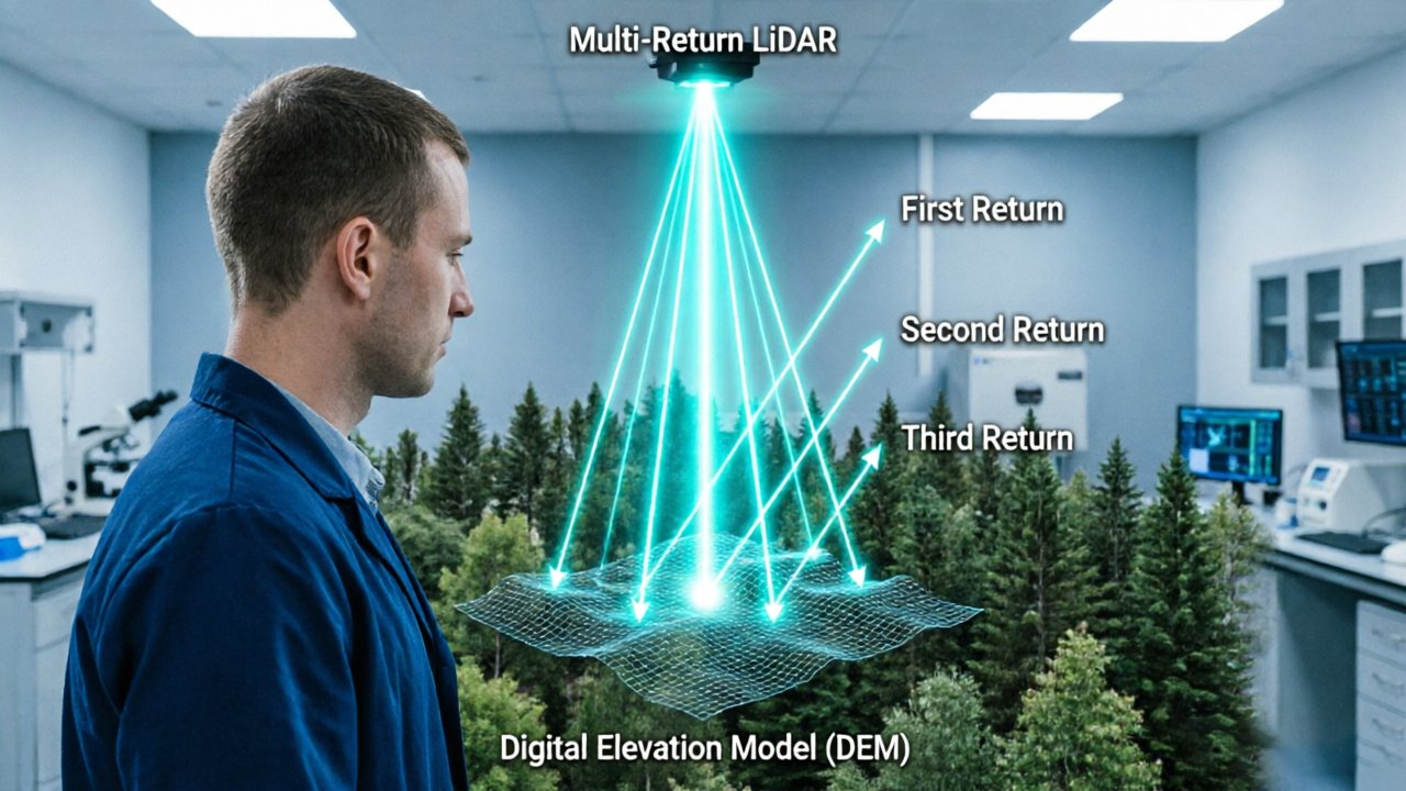
Multi-return LiDAR forestry applications depend on a deceptively simple principle: a single laser pulse can produce multiple distinct echoes as it travels through a forest canopy.
The laser doesn’t pass through leaves — it passes through the gaps between them. As the NOAA Office for Coastal Management explains, “the ability of LiDAR to ‘see through’ the canopy is not about the laser passing through solid leaves, but about the sensor’s ability to capture the energy that filters through small interstitial gaps.” Picture a single pulse fired downward into a dense stand of Douglas fir. The leading edge of that pulse strikes an upper branch and scatters — generating a first return. A portion of the remaining energy continues downward, hitting mid-story shrubs or understory limbs to produce one or more intermediate returns. What survives filters through to the forest floor, where the last return registers ground level. According to the USGS, discrete return LiDAR systems can capture multiple distinct returns per pulse — each one a discrete snapshot of a different vertical layer.
Discrete return systems record these peaks as individual point events, logging the precise time-of-flight for each. The sensor distinguishes between energy peaks by applying an amplitude threshold: when reflected intensity crosses that threshold, a return is logged and the clock resets to listen for the next peak. This process repeats until the pulse energy is exhausted or a maximum return count is reached.
Full-waveform LiDAR, by contrast, digitizes the entire returning signal as a continuous intensity curve. This approach is common in research and development contexts because it captures subtle sub-canopy features that discrete systems may miss. However, it generates significantly larger data volumes and requires more intensive post-processing.
Understanding how a pulse actually behaves inside a forest canopy sets the stage for a deeper question: once you have these layered returns, how do you separate ground truth from canopy structure?
Decoupling the Canopy: DSM vs. DEM in Dense Vegetation
Forest LiDAR’s core power lies in its ability to separate the ground from everything growing on top of it — producing distinct models that, together, reveal the full vertical structure of a forest stand.
Understanding how those models relate to each other starts with recognizing what each return actually represents. As covered in the previous section, a single laser pulse can interact with multiple surfaces as it travels downward through a canopy. The signals those interactions generate become the raw ingredients for three foundational data products.
The Digital Surface Model (DSM) is built primarily from first-return data. Every pulse that strikes the uppermost physical surface — the top of the canopy, an exposed branch, or open ground where no vegetation exists — contributes to this product. The DSM captures the highest intercepted elevation at any given geographic point, which in closed-canopy forests means it almost exclusively reflects treetop elevation rather than terrain.
The Digital Elevation Model (DEM) is the inverse: it represents ground truth. Constructed from last returns that penetrated all vegetative layers and struck bare earth, the DEM is a model of terrain independent of what grows on it. In practice, generating an accurate DEM beneath dense forest cover is among the most technically demanding tasks in forest LiDAR — and it’s precisely why single-return systems fall short.
The Canopy Height Model (CHM) emerges from the mathematical relationship between the two. As noted by the USGS, the difference between the DSM and DEM defines the CHM: subtract terrain elevation from surface elevation at each point, and the remainder is vegetation height. A pixel showing 35 meters in the CHM means the canopy rises 35 meters above the ground directly below it.
Intermediate returns — those that land neither at the very top nor the very bottom of the canopy — add a critical fourth dimension to this picture. These mid-story interactions map the fuel layer: shrubs, ladder fuels, and sub-canopy vegetation that fire behavior models depend on. Without intermediate returns, fuel layer mapping is essentially a blind estimate.
That vertical completeness is what makes multi-return forest LiDAR indispensable — though how much of it actually reaches the ground depends on canopy density, a problem the next section examines in depth.
The Limits of Penetration: Leaf Area Index (LAI) and Pulse Density
Dense forests don’t just challenge lidar forestry workflows — they actively resist them, and understanding why starts with a single metric: the Leaf Area Index.
LAI measures the total one-sided leaf area per unit of ground surface. A grassland might register an LAI of 1.0; a temperate mixed forest typically ranges between 3.0 and 5.0; a mature tropical rainforest can push LAI above 7.0. That number matters enormously because each unit of LAI represents another layer of interception opportunities for an outgoing laser pulse. According to the Journal of Remote Sensing, LiDAR pulses may penetrate canopies with an LAI of up to 6.0 while still returning sufficient ground points for reliable DEM construction — but beyond that threshold, the geometry of penetration starts to break down.
⚠️ Technical Warning: When LAI exceeds 6.0, ground return rates may not provide sufficient data for a continuous DEM surface. In practice, this means that even high-pulse-density acquisitions may produce gap-riddled bare-earth models in the most structurally complex forest types. Survey planning must account for this ceiling, not assume away from it.
Ground penetration rates in closed-canopy environments are sobering. Industry convention accepts 1–5% ground returns as the realistic yield from a single flight pass over dense forest — meaning that for every 100 pulses fired, only one to five reach bare earth. Spatial variability compounds this problem: leaf density is rarely uniform across a stand, so sensors must be selected and flight parameters optimized for the worst-case zones within the study area, not the average condition.
The blind spot problem emerges most sharply in multi-layered tropical forests, where a subcanopy layer of palms or dense understory shrubs intercepts last-return pulses before they complete their descent. These intermediate surfaces absorb energy that would otherwise generate ground returns, creating systematic voids in the point cloud that no amount of post-processing can fully recover.
Understanding where penetration fails is actually the first step toward overcoming it — and that’s precisely where advanced inversion techniques and intensity-weighted filtering begin to close the gap.
Advanced Inversion Techniques for Forest Parameter Accuracy
Raw point clouds are only as useful as the algorithms that transform them — and in digital elevation model forestry, inversion techniques determine whether biomass estimates are trustworthy or dangerously imprecise.
As covered in the previous sections, pulse density and canopy penetration define the ceiling of what’s possible. But once the returns are captured, the real computational work begins. Research published in the MDPI journal ‘Forests’ confirms that accurate inversion techniques are critical for converting raw point clouds into actionable forest metrics like volume and biomass — a step many workflows underestimate.
Inversion modeling typically works by fitting allometric relationships to height and density distributions within the point cloud, then projecting those relationships outward to estimate above-ground biomass. The challenge is that no two forest stands behave identically, which means generic inversion models can introduce systematic error when applied across heterogeneous landscapes.
Intensity-based weighting adds another dimension to this process. In terrestrial LiDAR specifically, return intensity — the energy reflected back to the sensor — varies by surface type, moisture content, and incidence angle. Weighting returns by intensity allows processors to differentiate between bark, foliage, and soil more reliably, sharpening the separation between true ground returns and low-lying understory vegetation.
That understory is where noise filtration becomes essential. Low-lying brush, fallen logs, and dense shrubs produce returns that sit just above the soil surface — close enough to mimic ground signals and corrupt the DEM if left unfiltered. A robust noise filtration pipeline typically includes:
- Statistical outlier removal to eliminate isolated returns well above or below the local surface trend
- Progressive morphological filtering to separate ground from non-ground returns based on slope thresholds
- Height-threshold masking to suppress returns below a defined minimum elevation offset from the provisional ground surface
- Iterative cloth simulation filtering (CSF) for complex terrain where slope-based methods struggle
Pulse frequency ties everything together. Higher repetition rates maintain point density across fast-moving airborne platforms, ensuring the inversion algorithms have enough spatial coverage to produce statistically stable biomass estimates — a prerequisite before any meaningful fusion with external datasets can begin.
The Power of Fusion: Combining LiDAR with Multispectral Sentinel-2 Data
LiDAR excels at measuring forest structure, but structure alone can’t tell you what’s growing — and that distinction matters enormously for accurate forest management.
A structurally perfect canopy height model is still incomplete without the spectral data to identify the species beneath it. Multi-return LiDAR captures height, density, and vertical layering with precision. What it can’t capture is the biochemical fingerprint that separates a Douglas fir from a lodgepole pine. Species carry fundamentally different carbon densities, growth rates, and ecological roles — and confusing them introduces compounding errors into any downstream biomass or carbon estimate.
That’s where Sentinel-2 multispectral imagery steps in. The European Space Agency’s open-access satellite captures 13 spectral bands, including red-edge and shortwave infrared channels that are strongly correlated with chlorophyll content, water stress, and canopy phenology. These signatures are invisible to lidar but critical for species discrimination. According to PMC / NCBI research, fusion of dense airborne LiDAR and multispectral Sentinel-2 data is now the leading method for high-accuracy forest mapping at scale — precisely because each dataset compensates for the other’s blind spots.
The fusion workflow typically follows four stages:
- Acquisition alignment — LiDAR point clouds and Sentinel-2 scenes are co-registered to a common coordinate reference system.
- Feature extraction — Structural metrics (canopy height, return density, gap fraction) are derived from LiDAR; spectral indices like NDVI and red-edge NDRE are pulled from Sentinel-2.
- Joint classification — Both feature sets feed a machine learning classifier trained on field-validated species and land-cover labels.
- Output validation — Classified maps are assessed against independent plot data to confirm accuracy before operational use.
For large-scale industrial forestry — where a single management unit can span hundreds of thousands of acres — this fusion approach delivers a meaningful return on investment. Operators gain species-resolved canopy maps that support harvest scheduling, disease monitoring, and carbon inventory, all from data sources that are either freely available or increasingly cost-competitive with traditional aerial surveys.
The practical question, of course, is what this fusion workflow actually looks like when the data hits a processing pipeline — which is exactly what the next section walks through.
Visualizing the Forest Floor: A Practical Demonstration
Watching a dense point cloud transform from a wall of vegetation into a clean forest floor model is one of the most instructive moments in LiDAR-based forestry work — and seeing it in action clarifies what separates usable data from noise.
[VIDEO EMBED: YellowScan technical walkthrough — LiDAR point cloud processing through forest canopy to ground surface]
The raw point cloud is rarely what you work with. When a LiDAR sensor fires pulses into a forest, the initial return data is a dense, layered mass of returns from canopy tops, mid-story branches, understory shrubs, and — if lidar pulse penetration is sufficient — the actual ground surface. In a raw visualization, these layers are often indistinguishable at a glance. Every surface that reflected energy appears as a point, and without classification, the ground is buried beneath thousands of competing returns.
Ground classification is where the real work begins. Effective LiDAR mapping through vegetation requires specific software filtering to isolate ground returns from low-lying scrub, a step that separates last returns consistent with ground-level geometry from everything above. Algorithms like progressive triangulated irregular network (TIN) densification evaluate each point’s spatial relationship to its neighbors, iteratively building upward from the lowest, most geometrically consistent returns to identify the true terrain surface.
The “stripping” step — the visual removal of all non-ground classified points — is where a technical walkthrough becomes genuinely compelling. As vegetation layers disappear from the visualization, the forest floor topology emerges: subtle ridgelines, drainage channels, root mounds, and terrain features that canopy reflections completely obscured. A clean ground point cloud should appear continuous, with no obvious gaps or floating clusters that indicate misclassified shrub returns. Irregular voids or elevated point anomalies are the signatures of a classification that needs refinement.
Understanding what clean data looks like on-screen is foundational — but achieving it consistently depends heavily on the hardware doing the initial capture. The sensor’s return-handling capability plays a decisive role long before any software touches the data.
Procurement Strategy: Selecting Sensors for High-Density Environments
Choosing the right LiDAR sensor for dense forest environments isn’t about picking the newest hardware — it’s about matching verified specs to the physics of canopy penetration.
The number of returns a sensor can record per pulse is the single most important specification for forestry applications. As ASPRS documents, multi-return systems distinguish between canopy top and forest floor by recording time-of-flight for multiple energy peaks — meaning a sensor limited to two returns will routinely miss ground hits in high-LAI stands where a five- or six-return system succeeds. Before any other spec comparison, this number needs to be confirmed, not assumed.
Key must-have specs when evaluating sensors for dense forest deployments:
- Minimum 4–6 return channels per pulse for reliable ground point extraction beneath closed canopies
- High pulse repetition rate (≥300 kHz) to maintain point density at UAV survey speeds
- Narrow beam divergence (≤0.5 mrad) for precise vertical separation between canopy layers
- Ingress protection rating (IP67 or higher) for rain, humidity, and debris tolerance in field conditions
- Operating temperature range suitable for both tropical and boreal environments if global R&D is planned
Mechanical vs. solid-state is the other axis that frequently trips up procurement teams. Mechanical sensors offer wide, configurable fields of view that suit complex terrain well, but their rotating assemblies are vulnerable to vibration and shock on rugged ground-based platforms. Solid-state designs trade some angular coverage for significantly greater durability — a real advantage when sensors are mounted on forest robots traveling over root systems and uneven ground.
The procurement landscape itself is shifting. Factory-direct suppliers are disrupting traditional high-margin distribution channels by offering triple-certified hardware — typically CE, FCC, and RoHS compliance — at significantly lower overhead. For R&D teams deploying sensors across multiple regulatory jurisdictions, that certification stack removes a substantial barrier to international fieldwork without requiring costly re-qualification through regional distributors.
These hardware fundamentals set the foundation for the key takeaways that follow — because the right sensor choice downstream determines whether your ground models are accurate or quietly compromised.
The Bottom Line: Key Takeaways for Forestry R&D
Multi-return LiDAR isn’t just a hardware upgrade — it’s the foundational requirement for any forest DEM workflow that demands ground-level accuracy.
Multi-return capability is the single most important differentiator when evaluating sensors for dense forest environments. In closed-canopy conditions, research published in the Journal of Remote Sensing confirms that only 1–5% of pulses typically reach the forest floor. Without the ability to resolve multiple discrete returns per pulse, that narrow signal window is wasted. A single-return sensor, regardless of pulse repetition rate or beam divergence, simply cannot reconstruct the vertical structure that ground filtering algorithms depend on.
LAI thresholds define the practical ceiling of LiDAR penetration. A common pattern across field deployments is that sensors without high-sensitivity receivers begin to lose ground-point density when Leaf Area Index climbs above 6.0. Beyond that threshold, even well-configured sensors require careful flight planning — lower altitude, reduced speed, and overlapping scan lines — to compensate. Acknowledging this ceiling isn’t defeatist; it’s how R&D teams allocate budget and acquisition effort realistically.
Data fusion is accelerating. Pairing LiDAR-derived structural data with multispectral sources like Sentinel-2 is becoming standard practice in forest inventory pipelines. LiDAR resolves vertical architecture; multispectral imagery resolves species composition and phenological state. Neither dataset alone captures the full picture. The convergence of these two streams is where the next generation of carbon quantification and biomass modeling is being built.
Procurement discipline compounds these technical gains. Sourcing sensors factory-direct reduces the vendor margin layers that inflate R&D overhead, and triple-certified hardware removes the compliance friction that slows deployment in regulated environments.
The questions most teams encounter aren’t always about strategy — they’re often operational and highly specific. The next section addresses exactly that.
Frequently Asked Questions About Forestry LiDAR
Multi-return LiDAR raises practical questions that matter before any fieldwork begins — here are the answers that shape smarter deployment decisions.
Does intensity-based weighting improve accuracy in terrestrial scans?
Yes, and it’s one of the more underutilized tools in ground-point filtering. Intensity-based weighting helps correct for the varying reflectivity of different tree species and ground types, which means wet soil, leaf litter, and bare rock don’t all get treated as equivalent surfaces. In practice, applying intensity thresholds before classification reduces false ground returns and tightens DEM accuracy noticeably.
Can LiDAR see through dense tropical jungle?
Partially — and that qualifier matters. Even high-pulse-density airborne systems struggle in closed-canopy tropical environments where multi-layered vegetation leaves very few vertical gaps. A key metric is pulse penetration rate: in the densest rainforests, fewer than 5–10% of pulses may reach the ground, making multi-return capture and aggressive last-return filtering crucial. Combining LiDAR with complementary ground-truthing data remains the most reliable approach.
What is the difference between a 3-return and 5-return sensor?
A 3-return sensor typically records the first, a single intermediate, and last return per pulse. A 5-return sensor captures up to five discrete returns, giving far greater vertical resolution through layered canopies. More returns generally mean better sub-canopy structure reconstruction — particularly valuable when modeling mid-story vegetation or separating shrub layers from true ground returns in complex forest types.
How do I filter out noise from low-lying bushes?
The standard workflow combines height thresholding with morphological filtering — setting a minimum ground-clearance threshold (often 0.3–0.5 m) and applying algorithms like Cloth Simulation Filtering (CSF) or Progressive TIN Densification to isolate true ground points. Classifying returns by height percentile before generating the DEM prevents shrub returns from contaminating the bare-earth surface. Review your point cloud in cross-section slices to ensure the filter boundary is correctly positioned before a full run.