There was a moment—somewhere around 2019—when a quiet consensus shifted inside the world’s top autonomous vehicle programs. The engineering argument that lidar sensors in autonomous vehicles were an expensive luxury, a temporary crutch until cameras and neural networks matured, collapsed under the weight of real-world data. Depth ambiguity, low-light failures, and the brutal physics of high-speed edge cases made one thing undeniable: vision alone cannot guarantee geometric certainty. And at Level 4 autonomy, uncertainty is not an option.
The global automotive LiDAR market is projected to grow from approximately $700 million in 2023 to over $4.5 billion by 2030—a compound annual growth rate of nearly 30%, according to Fortune Business Insights. That trajectory isn’t driven by optimism. It’s driven by safety mandates.
Think of this as the Engineer’s Letter: an open acknowledgment that early cost skepticism, while financially reasonable, underestimated one fundamental problem. Cameras interpret reflected light patterns and infer distance. LiDAR measures it. That distinction—inference versus measurement—is the difference between a system that performs well under test conditions and one that achieves geometric ground truth: a precise, centimeter-accurate, three-dimensional model of the vehicle’s immediate environment at every moment.
Geometric ground truth is the missing link in most current ADAS stacks. As McKinsey & Company notes, “for a vehicle to truly understand its environment in complex urban settings, sensor fusion is non-negotiable.” Without a reliable spatial anchor, downstream perception tasks—object classification, path planning, collision avoidance—are built on probabilistic sand.
The emergence of solid-state lidar has further accelerated this shift, bringing down unit costs while improving reliability and form factor for production vehicles. What was once a spinning rooftop sensor the size of a coffee can is becoming an integrated architectural component.
This guide walks through the complete implementation blueprint: from selecting the right optical foundation, through calibration, to fusion architecture. The first decision—and arguably the most consequential—starts with the wavelength your sensor emits.
Step 1: Selecting the Optical Foundation—Wavelengths and 4D Capabilities
As established in the previous section, vision-only perception has real ceiling limits. The logical next step is understanding precisely which automotive lidar sensors belong in your stack—and that decision starts at the physics level, with wavelength selection.
Wavelength Trade-offs: 905nm vs. 1550nm
The two dominant wavelength bands each carry meaningful engineering trade-offs that directly affect system design.
| Wavelength | Effective Range | Eye Safety | Cost Impact | Best Use Case |
|---|---|---|---|---|
| 905nm | Up to ~150m | Class 1 (with power limits) | Lower | Urban, cost-sensitive fleets |
| 1550nm | Up to ~300m | Inherently safer at higher power | Higher | Highway L4, adverse weather |
The 1550nm band allows higher optical output without exceeding eye-safe thresholds, enabling longer-range detection in rain or fog. According to SAE International, LiDAR provides its own light source, which means it delivers consistent 3D depth perception even in pitch-black environments or near-whiteout conditions—an advantage neither band abandons, but one that 1550nm sensors exploit more aggressively at distance. However, silicon photonics components at 1550nm carry roughly 2–3x the per-unit cost of 905nm alternatives, a factor that can’t be ignored in high-volume deployment planning.
The Rise of 4D LiDAR: Doppler as a Native Channel
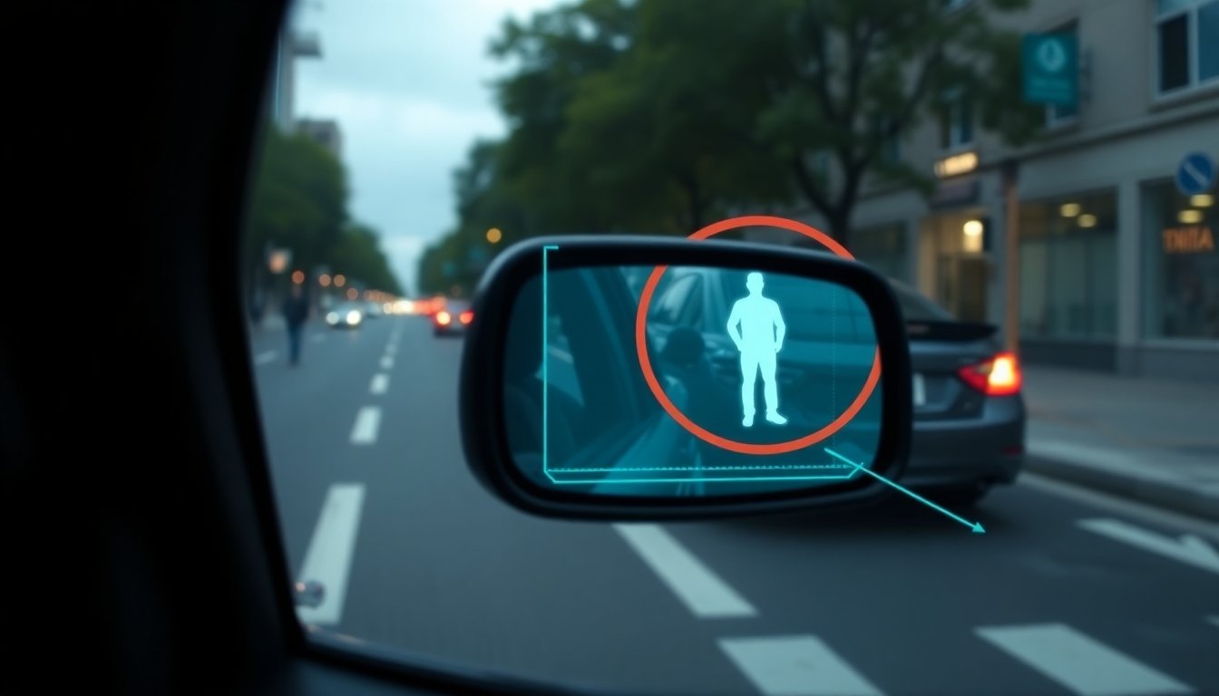
Listar4d (commonly called 4D LiDAR) represents a significant architectural step beyond conventional point cloud generation. By encoding instantaneous radial velocity data into each return point—using Doppler frequency shift—these sensors transform a static spatial snapshot into a dynamic scene with motion embedded at the point level. The practical result: a pedestrian stepping into a crosswalk registers not just where it is, but how fast it’s moving, in a single measurement cycle. This radically improves geometric ground truth accuracy by reducing the latency gap between perception and prediction layers. For L4 systems operating in dense urban intersections, that distinction isn’t incremental—it’s architectural.
Field of View and Point Density Requirements
FoV requirements differ sharply between deployment contexts:
- Urban scenarios demand wide horizontal FoV (≥120°) with strong near-field resolution to catch cyclists, pedestrians, and intersection geometry within 30m.
- Highway scenarios prioritize narrow, long-range FoV (60°–90° horizontal) with maximum range fidelity beyond 200m.
Verification Checkpoint: Before finalizing any sensor selection, confirm the device delivers a minimum of 1 million points per second. At high-speed highway navigation—where a vehicle closes 30 meters in under one second—anything below this threshold introduces dangerous sparse-sampling windows between scan cycles.
With wavelength, velocity encoding, and FoV resolved, the next critical decision concerns how the sensor physically generates those points—and whether its mechanical architecture can survive years of automotive-grade punishment.
Step 2: Architecture Choice—Solid-State vs. Mechanical Reliability
With the optical foundation established—wavelength selection, 4D capability, and field-of-view requirements locked in—the next critical decision is physical architecture. How the sensor moves (or doesn’t) determines whether it survives a decade of road deployment or fails three winters in.
The Mechanical Legacy and Why It’s Fading
Rotating LiDAR sensors dominated early autonomous development for good reason: 360-degree horizontal coverage, dense point clouds, and proven ranging performance. But passenger vehicle integration exposed a hard reality. These units sit tall on the roofline, creating aerodynamic drag and aesthetic problems. More critically, their spinning assemblies—bearings, motors, slip rings—accumulate wear with every road mile. High-frequency vibration from potholes and rough pavement accelerates that degradation in ways that controlled lab testing rarely captures.
The automotive industry doesn’t tolerate mechanical attrition at scale. When fleet deployment reaches thousands of vehicles operating continuously, even low failure rates create unsustainable maintenance burdens.
Solid-State Architectures: Three Paths Forward
Lidar technology for self-driving cars has matured into three distinct solid-state approaches, each with a different performance and reliability profile:
| Architecture | Mechanism | Practical Advantage |
|---|---|---|
| MEMS (Micro-Electromechanical Systems) | Tiny mirrors on silicon chips deflect laser pulses | Compact form factor; lower cost at volume |
| Flash LiDAR | Illuminates entire scene simultaneously | No scanning delay; excellent for near-field detection |
| OPA (Optical Phased Array) | Steers light electronically via phase modulation | No moving parts whatsoever; highest integration potential |
As noted by IEEE Xplore, solid-state LiDAR sensors are preferred for automotive use specifically because the absence of moving parts reduces mechanical failure caused by road shocks—a direct answer to the rotating sensor’s core vulnerability.
MTBF: The Number That Actually Matters
Mean Time Between Failures (MTBF) in a high-vibration automotive environment is the single most predictive reliability metric an architect should demand from any sensor vendor.
Rotating sensors typically target MTBF figures in the range of 1,000–2,000 hours under road conditions. Solid-state designs aim substantially higher because there’s no rotating mass to fatigue. However, MTBF claims vary widely depending on test conditions, so always request vibration profiles aligned with ISO 16750-3 (road vehicle environmental conditions).
Verification Checkpoint
Before approving any sensor for Level 4 deployment, confirm two non-negotiable specifications:
- IP69K rating — protects against high-pressure, high-temperature water jets common in vehicle wash environments
- Vibration resistance — validated against automotive-grade shock profiles, not consumer electronics standards
A sensor passing this checkpoint is architecturally ready. What it produces next—point clouds that need to be reconciled with camera data—takes us directly into the fusion layer, where geometric ground truth gets its first real test.
Step 3: Integrating Sensor Fusion—The ‘Ground Truth’ Layer
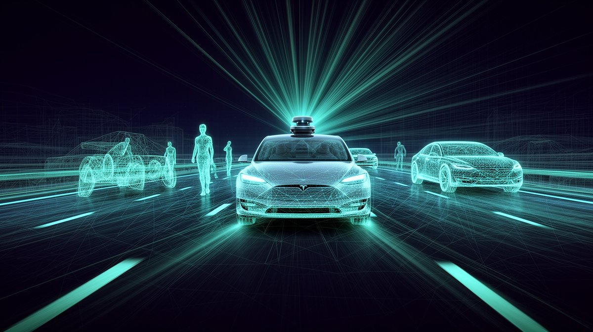
With architecture selected and your sensor array physically mounted, the real engineering challenge begins: teaching disparate data streams to speak a common language. Sensor fusion is where the full benefits of LiDAR sensors in cars become undeniable—transforming isolated point clouds, RGB frames, and radar returns into a unified, actionable world model.
Early Fusion vs. Late Fusion: Choosing Your Integration Point
The first decision is when to combine data streams. Early fusion merges raw inputs—LiDAR point clouds projected onto camera image planes—before any object classification occurs. This approach preserves maximum spatial detail and allows the neural network to learn cross-modal correlations from the ground up. Late fusion, by contrast, lets each sensor run its own detection pipeline independently, then reconciles outputs at the object-list level.
In practice, Level 4 systems increasingly favor hybrid fusion architectures, where LiDAR and camera data are early-fused for close-range scene understanding, while radar detections are late-fused for velocity confirmation at longer ranges. The Enhance-Fuse-Align principle formalizes this layered approach, demonstrating measurable improvements in detection consistency across varied traffic densities.
LiDAR as the Geometric Ground Truth Resolver
Camera systems excel at semantic richness—color, texture, lane markings—but they struggle with depth ambiguity. A flat billboard and a pedestrian at the same pixel coordinates look identical to a monocular model. LiDAR eliminates this ambiguity entirely. As McKinsey & Company notes, “LiDAR provides the precise geometric ground truth that radar and vision-only systems often lack in high-density traffic.”
The practical implementation involves point cloud projection: each LiDAR return is mapped onto the camera’s image plane using an extrinsic calibration matrix, attaching a verified depth value to every detected pixel region. Camera-identified objects that lack a corresponding LiDAR return are flagged as low-confidence detections requiring additional verification.
Handling Data Latency and Timestamp Alignment
Heterogeneous sensor arrays introduce a subtle but critical problem: sensors don’t capture the world simultaneously. A 10Hz LiDAR spinning at 100ms intervals combined with a 30fps camera creates temporal misalignment that compounds at highway speeds. The standard approach uses hardware-synchronized trigger signals and a software timestamp arbitration layer that interpolates sensor poses between capture events.
Step-by-step timestamp alignment process:
- Assign a hardware master clock (typically GPS-disciplined) to all sensor nodes
- Log capture timestamps at the hardware interrupt level, not software receipt
- Apply ego-motion compensation using IMU data to project older frames forward
- Reject frame pairs exceeding a configurable latency threshold (commonly 5–10ms)
[Insert Technical Video on Sensor Fusion Logic]
For deeper implementation detail, the RACF framework paper provides validated architectural patterns for distance-aware object detection exceeding 200 meters—a critical benchmark for highway-speed Level 4 operation.
Verification Checkpoint: Run your fusion pipeline against a labeled dataset containing objects at 200m+ range. Detection recall below 85% at that distance typically signals miscalibrated extrinsics or insufficient timestamp compensation—both correctable before moving to environmental stress testing.
With a validated fusion layer in place, the next challenge is ensuring that entire pipeline holds together when the real world turns hostile.
Step 4: Calibrating for Environmental Extremes
Even the most sophisticated sensor fusion stack from Step 3 can be undermined by one overlooked variable: the physical environment. Lidar sensors for ADAS must perform reliably not just on sunny California test tracks but in Minnesota blizzards, Arizona heat, and fog-blanketed coastal highways. Environmental calibration isn’t a post-deployment concern—it belongs in the architecture blueprint from day one.
Mitigating Weather Noise: Rain, Snow, and Fog
Precipitation introduces backscatter—photons reflecting off water droplets before ever reaching a target object—which manifests as dense noise clouds in raw point data. The standard mitigation approach combines intensity thresholding with temporal filtering: points that appear in only one or two consecutive frames and fall below a minimum return intensity are flagged as probable atmospheric artifacts and suppressed before object detection runs.
Fog presents the greatest challenge because its particle density closely mimics low-reflectivity surfaces. In practice, dual-return processing—capturing both the first and strongest return from a single pulse—allows the system to distinguish fog scatter from a solid obstacle behind it. Algorithms trained on worst-case visibility scenarios (typically below 50 meters) can reduce false-positive object detections by a significant margin, though the exact improvement depends heavily on wavelength selection established in Step 1.
Thermal Management: The -40°C to +85°C Operating Window
Automotive-grade sensors must meet the AEC-Q100 thermal stress standard, covering the full range from deep winter cold to engine-bay-adjacent heat. Temperature fluctuation causes mechanical expansion in optical housings, shifting beam divergence and introducing range error. The practical solution is onboard temperature compensation firmware: the sensor continuously reads an internal thermistor and applies real-time correction coefficients to range calculations, keeping accuracy within specification across the entire window. Validate this during bench testing by cycling the sensor through thermal extremes before road validation—failures caught in a thermal chamber are far cheaper than field recalls.
Self-Cleaning Mechanisms and Glare Verification
Lens contamination—road grime, salt spray, insect debris—is one of the most underestimated threats to sensor uptime. Integrated lens washers and heaters are no longer optional on production-grade systems; heaters prevent condensation and ice formation, while pressurized washers restore optical clarity without vehicle intervention.
Reliable autonomous operation depends on sensors that clean and stabilize themselves, because a contaminated lens degrades ground truth faster than any software bug.
Verification Checkpoint: To confirm the system correctly distinguishes ghost reflections from physical obstacles in high-glare conditions, conduct controlled testing against retroreflective surfaces under direct sunlight. As SAE International notes, unlike camera systems, LiDAR is unaffected by direct sunlight white-out conditions, making it a critical safety redundancy—but specular ghost returns from wet pavement or metallic barriers still require explicit filtering validation. Pass/fail criteria: zero unresolved ghost objects persisting beyond three consecutive frames at a standardized test distance.
With environmental resilience confirmed, the remaining practical questions—power budgets, interference management, and fleet longevity—are addressed directly in the FAQ below.
Frequently Asked Questions
What is the difference between 4D LiDAR and traditional 3D LiDAR?
Traditional 3D LiDAR captures spatial data across X, Y, and Z axes, producing dense point clouds that define object geometry. 4D LiDAR adds a fourth dimension: radial velocity, measuring the Doppler shift of returned laser pulses to determine how fast objects are moving relative to the sensor. In practice, this means a 4D system can distinguish a stationary pedestrian from one stepping into traffic—without waiting for multiple scan frames to confirm motion. For Level 4 systems, that latency reduction is operationally significant.
How does LiDAR handle interference from other vehicles’ sensors?
Crosstalk between LiDAR units is a real concern in dense autonomous vehicle deployments. Modern systems mitigate this through randomized pulse encoding and frequency modulated continuous wave (FMCW) techniques, which allow each sensor to distinguish its own returns from ambient laser noise. The Enhance-Fuse-Align architectural principle further recommends preprocessing pipelines that flag statistically anomalous returns before they enter the sensor fusion stack, preserving point cloud integrity even in high-traffic corridors.
Can LiDAR replace Radar entirely in Level 4 systems?
Not reliably—and this is a critical caveat. LiDAR excels at geometric resolution but degrades in heavy precipitation, where radar maintains velocity tracking performance. A common pattern in production L4 architectures is treating radar as the long-range velocity anchor and LiDAR as the geometric ground-truth layer. Removing radar entirely introduces single-point failure risk that conflicts with functional safety standards like ISO 26262.
What are the power consumption requirements for a typical automotive LiDAR suite?
A multi-unit LiDAR configuration—typically four to six sensors covering a 360-degree perimeter—draws between 30W and 100W total, depending on sensor type and resolution settings. Solid-state units generally consume less power than mechanical spinning designs. Engineers should budget additional thermal management overhead, particularly for roof-mounted units exposed to direct solar load during summer operation.
How do solid-state sensors improve the lifespan of autonomous fleets?
Mechanical LiDAR relies on rotating assemblies with bearings and motors—components subject to wear under continuous operation. Solid-state designs eliminate moving parts entirely, dramatically reducing failure rates. In practice, fleets transitioning to solid-state sensors report longer mean time between failures and lower maintenance intervals, which directly impacts total cost of ownership for commercial Level 4 deployments.
Implementing automotive LiDAR at the Level 4 standard demands more than capable hardware—it requires architectural discipline across sensor selection, fusion design, environmental calibration, and long-term fleet durability. The decisions made at each layer compound, and shortcuts at the sensor integration stage consistently surface as system-level failures later.
Sustainable autonomy isn’t built on any single sensor—it’s built on the disciplined orchestration of every data stream feeding the perception stack.
Explore the full range of automotive perception hardware available for your next deployment in our complete sensor catalog.
Key Takeaways
- Urban scenarios demand wide horizontal FoV (≥120°) with strong near-field resolution to catch cyclists, pedestrians, and intersection geometry within 30m.
- Highway scenarios prioritize narrow, long-range FoV (60°–90° horizontal) with maximum range fidelity beyond 200m.
- IP69K rating — protects against high-pressure, high-temperature water jets common in vehicle wash environments
- Vibration resistance — validated against automotive-grade shock profiles, not consumer electronics standards
- Assign a hardware master clock (typically GPS-disciplined) to all sensor nodes